5. Population Model Evaluation

Overview

This tutorial demonstrates how to evaluate and compare population model results across different species profiles and parameter sets. Understanding the sensitivity of model outputs to input parameters is essential for identifying which vital rates matter most and where uncertainty in the data translates into uncertainty in population projections.

We cover two complementary approaches:

Profile comparison — Swap in different life cycle profiles for the same study system and compare spawner abundance trajectories. This shows how demographic differences between populations (or parameter uncertainty between data sources) affect projected outcomes.
LTRE range analysis — Use Monte Carlo sampling and Partial Rank Correlation Coefficients (PRCC) to systematically quantify which parameters have the greatest influence on population growth rate (lambda).

Prerequisites

Before starting this tutorial, you should:

Complete Tutorial 3: Population Model Overview to understand life cycle profiles, density dependence, and the population model functions
Complete Tutorial 4: Population Model Batch Run for experience with batch processing
Review the Life Cycle Model chapter of the CEMPRA Guidance Document for detailed parameter descriptions

Part 1: Comparing Species Profiles

In this section we use stressor-response and stressor-magnitude values from the Nanaimo River Chinook salmon dataset, but swap out the life cycle profile to compare how different parameter sets affect population projections. The following populations are available as example profiles:

Nanaimo River Summer Chinook (vital rates from DFO-RAMs)
Chehalis River Spring/Fall Chinook in coastal Washington (parameters from Beechie et al., 2021)
Columbia River Chinook from Wenatchee River (parameters from Honea et al., 2009)
Nicola River spring-run Chinook from the interior of BC (DFO-RAMs 2021)

Load Input Data

We load the Nanaimo River stressor data and habitat capacities as a starting point. The life cycle profile will be swapped out in subsequent sections.

library(CEMPRA)
library(ggplot2)
library(dplyr)

# Set seed for reproducibility
set.seed(123)

# Stressor-magnitude workbook (location-specific stressor values)
fname <- system.file("extdata/nanaimo/stressor_magnitude_nanaimo.xlsx", package = "CEMPRA")
dose <- StressorMagnitudeWorkbook(filename = fname)
dose$SD <- 0  # Remove stochastic variation in stressor magnitudes for cleaner comparison

# Stressor-response workbook (dose-response curves)
fname <- system.file("extdata/nanaimo/stressor_response_nanaimo.xlsx", package = "CEMPRA")
sr_wb_dat <- StressorResponseWorkbook(filename = fname)

# Location and stage-specific habitat capacities
filename <- system.file("extdata/nanaimo/habitat_capacities_nanaimo.csv", package = "CEMPRA")
habitat_capacities <- read.csv(filename, stringsAsFactors = FALSE)

# Life cycle parameters (starting with Nanaimo summer Chinook)
filename_lc <- system.file("extdata/nanaimo/species_profiles/nanaimo_comp_ocean_summer.csv", package = "CEMPRA")
life_cycle_params <- read.csv(filename_lc)

Target Populations

The habitat capacities file lists the target populations. The density-dependent constraints estimate capacities in the absence of any stressors and assume that 100% of the stream area is suitable for spawning (e.g., gravel coverage = 100% and spawning suitability = 100%). Specific stressors targeting capacities will reduce these numbers to more realistic estimates.

print(habitat_capacities)
#>   HUC_ID           NAME k_stage_0_mean k_stage_Pb_1_mean k_stage_B_mean
#> 1      1     Fall Lower         627594                NA          38073
#> 2      2 Summer - Lower        1247555                NA          15384
#> 3      3 Summer - Upper         913589                NA          20943

# Focus analysis on Lower Nanaimo River Summer-Run Chinook (HUC_ID = 2)
HUC_ID <- 2

Run the Population Model

We run the population model using output_type = "full" (the default) to access the complete output structure, including stage-specific abundances for each Monte Carlo simulation. This is necessary for extracting spawner counts by age class.

data <- PopulationModel_Run(
  dose = dose,
  sr_wb_dat = sr_wb_dat,
  life_cycle_params = life_cycle_params,
  HUC_ID = 2,                           # Lower Summer-run Chinook
  n_years = 200,                         # Extended projection to see long-term dynamics
  MC_sims = 5,                           # Monte Carlo simulations
  habitat_dd_k = habitat_capacities      # Location-specific carrying capacities
)

# The "full" output is a nested list
names(data)
#> [1] "ce"       "baseline" "MC_sims"

# 5 Monte Carlo replicates for the CE scenario
length(data$ce)
#> [1] 5

# Each replicate contains population vectors, matrices, and diagnostics
names(data$ce[[2]])
#> [1] "pop"     "N"       "lambdas" "info"

# Stage-specific abundance over time (last 6 years of replicate 2)
tail(round(data$ce[[2]]$N, 0))
#>           K1   K2   K3  K4  K5  K6  K7
#> [196,] 70405 3911 2271 403 209 214 292
#> [197,] 22547 3119 2102 728 226 474 163
#> [198,] 42406  850 1535 652 352 882 572
#> [199,] 91737 1305  476 471 105 630 528
#> [200,] 57121 4052  641 158 147 210 389
#> [201,] 77627 3027 2307 192 508 259 127

Visualize the Time Series Projections

The pop_model_get_spawners() helper function extracts spawner abundance from the full output, combining results across Monte Carlo simulations into a clean data frame. We filter out the first 50 years of “burn-in” to focus on the equilibrium dynamics.

# Extract spawner abundance from the full output
spawners <- pop_model_get_spawners(
  data = data,
  life_stage = "spawners",
  life_cycle_params = life_cycle_params
)

head(spawners)
#>   location_id rep_id year spawners
#> 1           2      1    1    15384
#> 2           2      1    2     1111
#> 3           2      1    3     1262
#> 4           2      1    4     2256
#> 5           2      1    5     1989
#> 6           2      1    6     1359

# Summarize across simulations: mean and SD of spawners per year
summary_data <- spawners %>%
  filter(year > 50) %>%
  group_by(location_id, year) %>%
  summarize(
    mean_spawners = mean(spawners),
    sd_spawners = sd(spawners),
    .groups = "drop"
  )

# Plot mean spawner trajectory with uncertainty ribbon
ggplot(summary_data, aes(x = year, y = mean_spawners)) +
  geom_line(color = "blue", linewidth = 1) +
  geom_ribbon(
    aes(ymin = mean_spawners - sd_spawners, ymax = mean_spawners + sd_spawners),
    fill = "blue", alpha = 0.2
  ) +
  labs(title = "Spawner Abundance Over Time",
       subtitle = "Nanaimo River Summer Chinook (mean +/- 1 SD across simulations)",
       x = "Simulation Year", y = "Number of Spawners (N)") +
  theme_bw() +
  theme(legend.position = "bottom")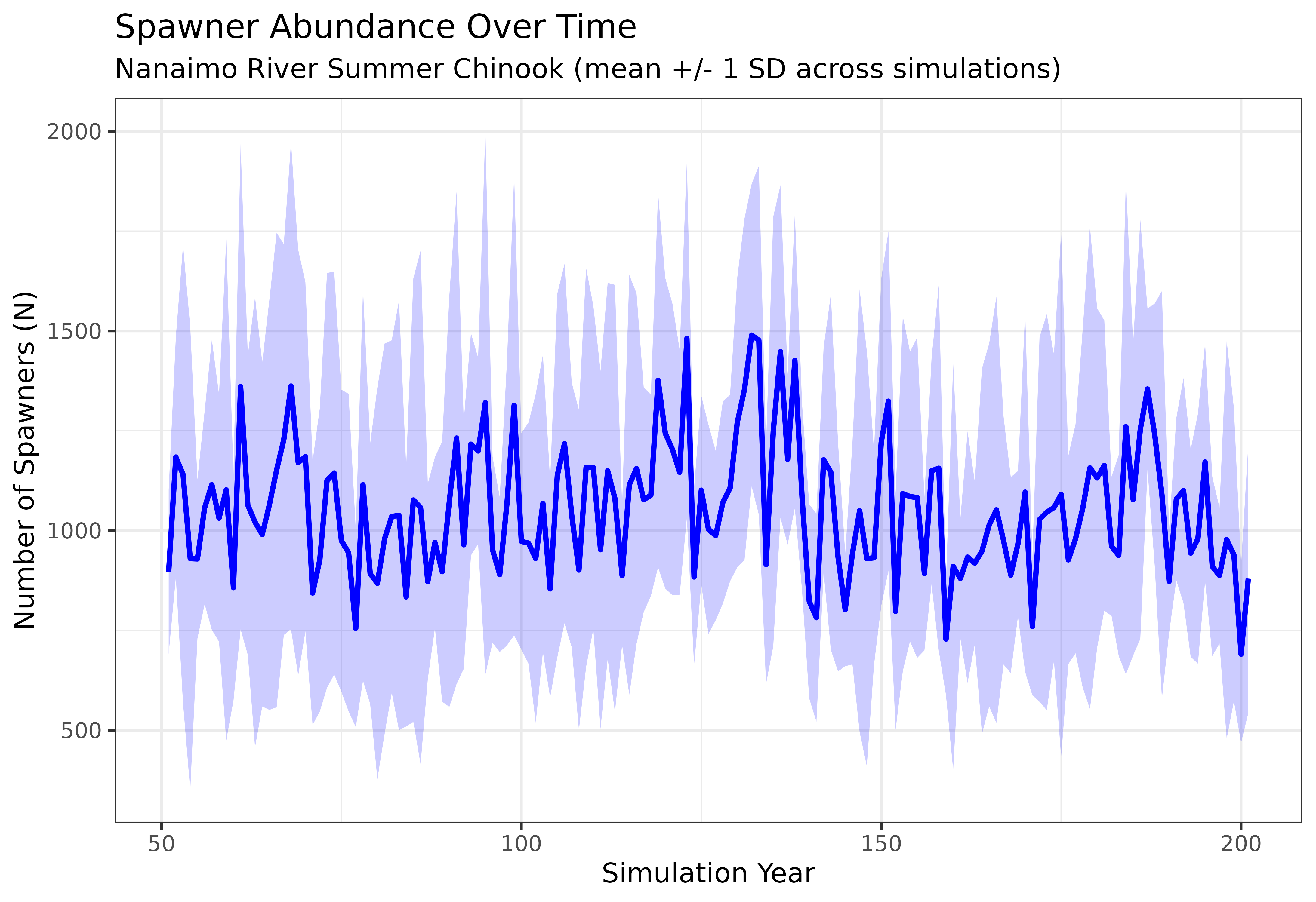

The blue ribbon shows the inter-simulation variability in spawner abundance. A wide ribbon indicates high stochastic variability, while a narrow ribbon suggests the population dynamics are relatively stable across replicates. Both the mean trajectory and the width of the ribbon are informative — they tell you about the expected population size and the uncertainty around that expectation.

Part 2: LTRE Range Analysis (Global Sensitivity)

A Life Table Response Experiment (LTRE) identifies which demographic parameters have the greatest influence on population growth rate. The pop_model_ltre_range() function implements an uncertainty-based LTRE approach: rather than perturbing each parameter by a fixed amount, it samples from user-defined probability distributions and uses Partial Rank Correlation Coefficients (PRCC) to quantify the relationship between each parameter and lambda (the population growth rate).

This approach is particularly valuable for:

Identifying key vital rates — Which parameters, given their realistic range of uncertainty, have the most influence on whether the population grows or declines?
Prioritizing data collection — Parameters with high PRCC and wide uncertainty ranges are candidates for additional field studies.
Understanding risk — What is the probability that lambda falls below 1 (population decline) given current parameter uncertainty?

See the Life Cycle Model chapter of the guidance document for more background on the vital rates and their biological interpretation.

Preparing the Input File

The LTRE range analysis requires an extended life cycle CSV with additional columns that specify how each parameter should be sampled:

Column	Description
`Parameters`	Human-readable parameter description
`Name`	Parameter code used by the model (e.g., `SE`, `surv_1`)
`Value`	Central value (used as mean for normal/beta, mode for PERT)
`Notes`	Optional notes or data sources
`Test_Parameter`	`TRUE` to include in sensitivity analysis, `FALSE` to hold fixed
`Distribution`	Sampling distribution: `"normal"`, `"beta"`, or `"pert"`
`SD`	Standard deviation (required for normal and beta distributions)
`Low_Limit`	Lower bound for sampling
`Up_Limit`	Upper bound for sampling

Parameters marked Test_Parameter = FALSE (e.g., Nstage, compensation ratios) are held constant across all simulations. Only parameters marked TRUE are sampled and included in the PRCC analysis.

# Load the example LTRE input file
lc_file <- system.file("extdata/ltre/life_cycles_input_ltre.csv", package = "CEMPRA")
life_cycle_ltre <- read.csv(lc_file)

# View the first few rows to see the extended column structure
head(life_cycle_ltre[, c("Name", "Value", "Test_Parameter", "Distribution", "SD", "Low_Limit", "Up_Limit")], 10)
#>          Name Value Test_Parameter Distribution      SD Low_Limit Up_Limit
#> 1      Nstage     5          FALSE                   NA        NA       NA
#> 2  anadromous  TRUE          FALSE                   NA        NA       NA
#> 3           k  5000          FALSE                   NA        NA       NA
#> 4      events     1          FALSE                   NA        NA       NA
#> 5       eps_3  3000           TRUE       normal 250.000     5e+02    5e+03
#> 6       eps_4  4000           TRUE       normal 500.000     1e+03    6e+03
#> 7       eps_5  4810           TRUE       normal 600.000     1e+03    7e+03
#> 8         int     1          FALSE                   NA        NA       NA
#> 9          SE   0.2           TRUE         beta   0.036     5e-02    8e-01
#> 10         S0   0.3           TRUE         pert      NA     2e-02    4e-01

Note how structural parameters (Nstage, anadromous, k) and compensation ratios (cr_E, cr_0, etc.) have Test_Parameter = FALSE — these define the model structure and are not varied. Vital rates like survival (SE, S0, surv_1), fecundity (eps_3, eps_4), and maturity (mat_3, mat_4) are marked TRUE and will be sampled.

Running the Analysis

The pop_model_ltre_range() function draws n_samples Monte Carlo samples from the specified distributions, builds a population matrix for each sample, calculates lambda, and then computes PRCC values to rank parameter importance.

# Run the LTRE range analysis
result <- pop_model_ltre_range(
  life_cycle_params = life_cycle_ltre,
  n_samples = 1000,   # Number of Monte Carlo samples
  seed = 42           # For reproducibility
)

Interpreting the Results

The function returns a list with several components:

PRCC Rankings

The prcc_rankings data frame shows each parameter’s Partial Rank Correlation Coefficient with lambda, sorted by absolute importance. A higher absolute PRCC means the parameter has a stronger influence on population growth rate, after controlling for the effects of all other parameters.

# Top 10 most influential parameters
head(result$prcc_rankings, 10)
#>    parameter       prcc       p_value   abs_prcc
#> 1     surv_2 0.92516735  0.000000e+00 0.92516735
#> 2     surv_1 0.85030554 1.797481e-280 0.85030554
#> 3         S0 0.49899747  4.442597e-64 0.49899747
#> 4     surv_3 0.49415174  1.086775e-62 0.49415174
#> 5         SE 0.33647155  6.820150e-28 0.33647155
#> 6     smig_4 0.23460315  5.706666e-14 0.23460315
#> 7      eps_4 0.23067286  1.522097e-13 0.23067286
#> 8         SR 0.10415170  9.723027e-04 0.10415170
#> 9        u_4 0.08883449  4.935108e-03 0.08883449
#> 10    surv_4 0.08714708  5.822138e-03 0.08714708

Positive PRCC values indicate that increasing the parameter increases lambda (e.g., survival rates), while negative values indicate the opposite. The p_value column tests whether the correlation is statistically significant.

Lambda Distribution Summary

The lambda_summary provides key statistics about the distribution of population growth rates across all Monte Carlo samples:

# Lambda summary statistics
result$lambda_summary
#> $mean
#> [1] 1.317683
#> 
#> $median
#> [1] 1.155925
#> 
#> $sd
#> [1] 0.5336746
#> 
#> $quantiles
#>      2.5%        5%       10%       25%       50%       75%       90%       95% 
#> 0.6269477 0.6823021 0.7754471 0.9415404 1.1559250 1.6144898 2.1765025 2.4200475 
#>     97.5% 
#> 2.6147206 
#> 
#> $prob_lambda_gt_1
#> [1] 0.684
#> 
#> $prob_lambda_lt_1
#> [1] 0.316
#> 
#> $n_valid
#> [1] 1000
#> 
#> $n_failed
#> [1] 0

Key values to look for:

prob_lambda_gt_1 — The probability that the population is growing. Values near 1.0 suggest the population is likely viable; values near 0 suggest likely decline.
prob_lambda_lt_1 — The probability of population decline.
median — The central estimate of lambda. Values above 1.0 indicate growth, below 1.0 indicate decline.

Lambda Distribution

A histogram of lambda values across all samples shows the full range of possible growth rates given parameter uncertainty. The vertical black line marks lambda = 1 (stable population); the red dashed line marks the median.

# How many simulations had negative growth rates (lambda < 1)?
pct_decline <- round(sum(result$samples$lambda < 1) / nrow(result$samples) * 100, 1)

hist(result$samples$lambda,
     breaks = 40, col = "steelblue", border = "white",
     main = "Distribution of Lambda Across Monte Carlo Samples",
     xlab = "Lambda (population growth rate)",
     sub = paste0(pct_decline, "% of samples have lambda < 1"))
abline(v = 1, col = "black", lty = 1, lwd = 2)
abline(v = result$lambda_summary$median, col = "red", lty = 2, lwd = 2)
legend("topright",
       legend = c("Lambda = 1 (stable)", paste("Median =", round(result$lambda_summary$median, 3))),
       lty = c(1, 2), lwd = 2, col = c("black", "red"), cex = 0.8)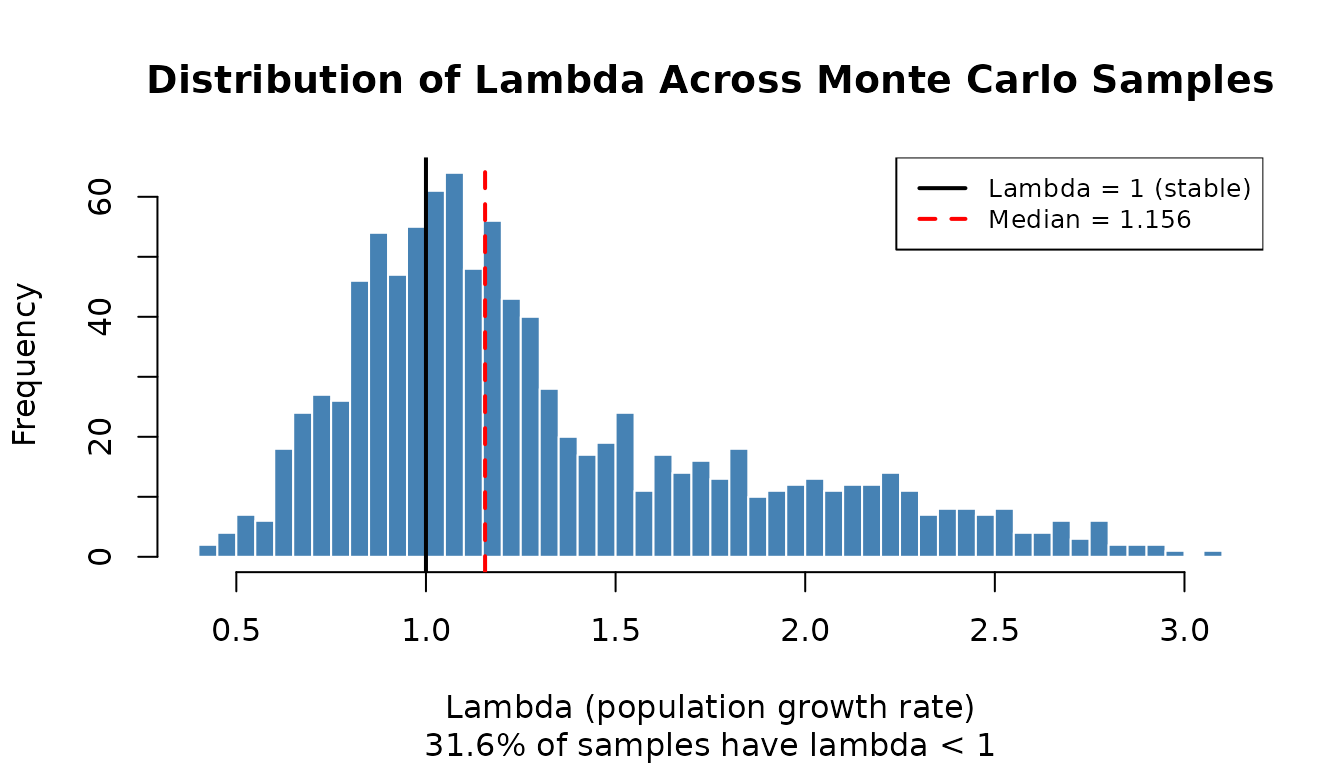

PRCC Sensitivity Bar Chart

A horizontal bar chart ranks parameters by their absolute PRCC value, with colors indicating statistical significance. Parameters at the top of the chart are the strongest drivers of population growth rate.

# Prepare data for plotting
prcc_data <- result$prcc_rankings

# Reorder factor levels by absolute PRCC (highest at top)
prcc_data$parameter <- factor(prcc_data$parameter, levels = rev(prcc_data$parameter))

# Define significance based on p-value
prcc_data$significant <- prcc_data$p_value < 0.01

ggplot(prcc_data, aes(x = abs_prcc, y = parameter, fill = significant)) +
  geom_col(width = 0.7) +
  scale_fill_manual(
    values = c("TRUE" = "steelblue", "FALSE" = "coral"),
    labels = c("TRUE" = "Significant (p < 0.01)", "FALSE" = "Not significant (p > 0.01)"),
    name = ""
  ) +
  scale_x_continuous(limits = c(0, 1), breaks = seq(0, 1, 0.25)) +
  labs(x = "Absolute PRCC with Lambda",
       y = "Model Parameter",
       title = "Parameter Sensitivity Rankings (LTRE Range Analysis)",
       subtitle = paste0("Based on ", result$metadata$n_samples, " Monte Carlo samples")) +
  theme_bw() +
  theme(panel.grid.major.y = element_blank(),
        panel.grid.minor = element_blank(),
        legend.position = "bottom")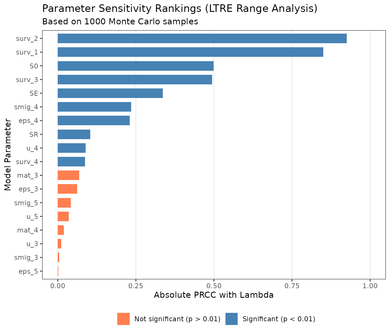

Parameters with high PRCC values and wide uncertainty ranges are the best candidates for additional data collection — reducing uncertainty in these parameters will have the greatest effect on the precision of your population projections.

Next Steps

For additional guidance, see the CEMPRA Documentation:

Life Cycle Profiles — detailed parameter descriptions for building custom species profiles
Stochastic Simulations — background on variance and correlation parameters
Density-Dependent Constraints — compensation ratios, Beverton-Holt, and Hockey-Stick options
Case Studies — real-world applications of the CEMPRA framework

References

Beechie, T. et al. (2021). Restoring salmon habitat for a changing climate. River Research and Applications, 37(4), 601-625.
Honea, J. M. et al. (2009). Evaluating habitat effects on population status: influence of habitat restoration on spring-run Chinook salmon. Freshwater Biology, 54(7), 1576-1592.

2026-04-22