Overview
This tutorial provides an introduction to the Joe Model, a core component of the CEMPRA (Cumulative Effects Model for Prioritizing Recovery Actions) framework. By the end of this tutorial, you will understand how to:
- Import stressor-response and stressor-magnitude data
- Calculate system capacity for individual stressors
- Run the full Joe Model to assess cumulative effects across multiple stressors
What is the Joe Model?
The Joe Model is a cumulative effects assessment tool that quantifies how multiple environmental stressors combine to affect the capacity of a system to support a target species or ecosystem function.
The model works by:
- Defining stressor-response relationships: How does each environmental stressor (e.g., temperature, sediment, flow alteration) affect system capacity?
- Measuring stressor magnitudes: What are the current levels of each stressor at locations of interest?
- Combining effects: How do multiple stressors interact to produce a cumulative effect on the system?
The output is a system capacity score (0-100%) representing the relative ability of each location to support the target species, given current stressor conditions.
Understanding the Input Data
The Joe Model requires two Excel workbooks as input:
| Workbook | Purpose |
|---|---|
| Stressor-Response Workbook | Defines how each stressor affects system capacity (the dose-response curves) |
| Stressor-Magnitude Workbook | Contains measured or estimated stressor levels at each location |
These two workbooks work together: the stressor-response workbook tells us how bad a given stressor level is, while the stressor-magnitude workbook tells us what the stressor levels actually are at each location.
Stressor-Response Workbook
The stressor-response workbook defines the relationship between environmental conditions and system capacity. Think of it as answering the question: “If temperature is 18°C, what percentage of optimal habitat capacity remains?”
Workbook Structure
The stressor-response Excel workbook must follow a standardized format with:
- A Main worksheet listing all stressors and their properties
- Individual worksheets for each stressor containing the dose-response curve data
The Main Worksheet
The Main worksheet serves as a master index of all
stressors in your analysis. Here’s an example of what it looks like:
#>      Stressors Stressor_cat Interaction Linked Stress_Scale   Function
#> 1     Aug_flow     Aug_flow     Minimum      A       linear continuous
#> 2 Barrier_dams Barrier_dams          NA     NA       linear       step
#> 3         BKTR         BKTR          NA     NA       linear continuous
#> 4     Feb_flow     Feb_flow     Minimum      A       linear continuous
#> 5    Foot_flow    Foot_flow          NA     NA       linear continuous
#>   Life_stages Parameters Units     Model
#> 1       adult       <NA>    NA Joe Model
#> 2       adult       <NA>    NA Joe Model
#> 3       adult       <NA>    NA Joe Model
#> 4       adult       <NA>    NA Joe Model
#> 5       adult       <NA>    NA Joe Model
Each row represents one stressor, with the following columns:
| Column | Description |
|---|---|
| Stressors | Unique name for the stressor (must match worksheet name exactly) |
| Stressor_cat | Category grouping (used in population model for linking to vital rates) |
| Interaction | How this stressor combines with others: NA/blank
(multiplicative), Additive, or Minimum
|
| Linked | For minimum interactions, which stressor this one is linked to |
| Stress_Scale | Scale of the x-axis: linear or
logarithmic
|
| Function | Curve type: continuous (smooth interpolation) or
step (discrete thresholds) |
| Life_stages | Which life stage this stressor affects (e.g., fry_parr,
adult) |
| Parameters | What the stressor affects: blank/NA for system
capacity, or survival/capacity for vital
rates |
Stressor-Response Curve Worksheets
After the Main worksheet, each stressor must have its own worksheet containing the dose-response data. The worksheet name must exactly match the stressor name in the Main sheet.
Each dose-response curve defines how system capacity changes across a range of stressor values:
| Temperature (°C) | Mean System Capacity (%) | SD | Lower Limit | Upper Limit |
|---|---|---|---|---|
| 12 | 60 | 15 | 10 | 80 |
| 14 | 80 | 10 | 30 | 95 |
| 16 | 100 | 10 | 40 | 100 |
| 18 | 95 | 10 | 40 | 100 |
| 20 | 30 | 5 | 0 | 50 |
| 22 | 15 | 3 | 0 | 30 |
| 24 | 0 | 0 | 0 | 0 |
| 26 | 0 | 0 | 0 | 0 |
| 28 | 0 | 0 | 0 | 0 |
The columns are:
| Column | Description |
|---|---|
| Stressor values | The first column contains raw stressor values (e.g., temperature in °C) |
| Mean System Capacity | Expected system capacity (0-100%) at each stressor level |
| SD | Standard deviation representing uncertainty in the relationship |
| low.limit / up.limit | Absolute bounds for the system capacity (used to constrain random sampling) |
Visualizing the Dose-Response Curve
The figure below illustrates how to interpret a stressor-response curve. The optimal temperature for this species is around 16°C (100% capacity). As temperature increases beyond the optimum, capacity declines rapidly, reaching 0% at temperatures above 24°C.
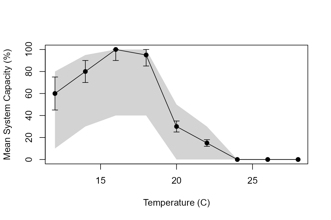
Example stressor-response curve showing how temperature affects system capacity. Error bars show standard deviation; grey shading shows the allowable range.
Key points about the uncertainty:
- The error bars (standard deviation) represent natural variability or uncertainty in the relationship
- The grey shading shows the absolute bounds - system capacity values will never fall outside this range
- During Monte Carlo simulations, values are sampled from this distribution to propagate uncertainty through the analysis
Loading the Stressor-Response Workbook
Use the StressorResponseWorkbook() function to import
and validate your data:
# Load the example stressor-response workbook included with CEMPRA
filename_sr <- system.file("extdata", "stressor_response_fixed_ARTR.xlsx", package = "CEMPRA")

# Import and validate the workbook
sr_wb_dat <- StressorResponseWorkbook(filename = filename_sr)

# The function returns a list with two components:
names(sr_wb_dat)
#> [1] "main_sheet"     "stressor_names" "pretty_names"   "sr_dat"
The returned object contains:
-
main_sheet: The Main worksheet data as a data frame -
sr_dat: A list of data frames, one for each stressor’s dose-response curve
Stressor-Magnitude Workbook
While the stressor-response workbook defines how stressors affect the system, the stressor-magnitude workbook tells us what the actual stressor levels are at each location.
This workbook contains location-specific measurements or estimates of each stressor, along with uncertainty bounds.
Workbook Structure
| HUC_ID | NAME | Stressor | Stressor_cat | Mean | SD | Distribution | Low_Limit | Up_Limit | Comments |
|---|---|---|---|---|---|---|---|---|---|
| 1702010107 | Example Location | Aug_flow | Aug_flow | 100 | 0 | normal | 100 | 0 | NA |
| 1702010107 | Example Location | Barrier_dams | Barrier_dams | 0 | 0 | normal | 0 | 5 | NA |
| 1702010107 | Example Location | BKTR | BKTR | 0 | 0 | normal | 0 | 100 | NA |
| 1702010107 | Example Location | Feb_flow | Feb_flow | 100 | 0 | normal | 100 | 0 | NA |
Each row represents one stressor at one location:
| Column | Description |
|---|---|
| HUC_ID | Unique numeric identifier for the location (originally Hydrological Unit Code, but can be any ID system) |
| NAME | Human-readable location name (for display purposes) |
| Stressor | Stressor name (must exactly match the stressor-response workbook) |
| Stressor_cat | Stressor category (must match the stressor-response workbook) |
| Mean | Mean/expected value of the stressor at this location |
| SD | Standard deviation representing measurement uncertainty or natural variability |
| Distribution | Sampling distribution: normal or
lognormal
|
| Low_Limit / Up_Limit | Bounds for the stressor values (prevents unrealistic samples) |
Loading the Stressor-Magnitude Workbook
Use the StressorMagnitudeWorkbook() function to import
your location data:
# Load the example stressor-magnitude workbook
filename_rm <- system.file("extdata", "stressor_magnitude_unc_ARTR.xlsx", package = "CEMPRA")

# Import the workbook - note that you specify which scenario worksheet to use
smw <- StressorMagnitudeWorkbook(filename = filename_rm, scenario_worksheet = "natural_unc")

# Preview the column names
names(smw)
#>  [1] "HUC_ID"       "NAME"         "Stressor"     "Stressor_cat" "Mean"
#>  [6] "SD"           "Distribution" "Low_Limit"    "Up_Limit"     "Comments"
Tip: The stressor-magnitude workbook can contain multiple scenario worksheets (e.g., “current”, “restored”, “future_climate”). This allows you to compare system capacity under different management scenarios without creating multiple files.
Calculating System Capacity
Now that we understand the input data, let’s calculate system capacity. We’ll start with a single stressor to understand the mechanics, then run the full model with all stressors.
A note on reproducibility: The Joe Model relies on Monte Carlo simulation, so results will differ slightly each time you run it. To get reproducible results (useful for debugging or verifying your setup), set a random seed before any model calls:
set.seed(123)Step 1: Generate Mean Response Curves
Before calculating system capacity, we need to process the
stressor-response data into interpolated curves. The
mean_Response() function creates smooth curves from the
discrete data points in your worksheets:
# Create interpolated response curves for all stressors
mean.resp.list <- mean_Response(
  n.stressors = nrow(sr_wb_dat$main_sheet),
  str.list = sr_wb_dat$sr_dat,
  main = sr_wb_dat$main_sheet
)
This creates a list of response functions that can convert any stressor value to a system capacity score.
Step 2: Calculate Capacity for a Single Stressor
Let’s calculate system capacity for temperature at a hypothetical location. This helps illustrate what the model is doing before we run the full analysis.
# Extract data for the "Temperature_adult" stressor
f.main.df <- sr_wb_dat$main_sheet[which(sr_wb_dat$main_sheet$Stressors == "Temperature_adult"), ]
f.stressor.df <- sr_wb_dat$sr_dat[["Temperature_adult"]]
f.mean.resp.list <- mean.resp.list[[which(sr_wb_dat$main_sheet$Stressors == "Temperature_adult")]]

# Create sample data for a hypothetical location
# Mean temperature = 14°C, SD = 3°C
smw_sample <- data.frame(
  HUC_ID = 0,
  NAME = "Example Location",
  Stressor = "Temperature_adult",
  Stressor_cat = "Temperature",
  Mean = 14,
  SD = 3,
  Distribution = "normal",
  Low_Limit = 4,
  Up_Limit = 20
)

# Calculate system capacity with 100 Monte Carlo simulations
test_sc <- SystemCapacity(
  f.dose.df = smw_sample,
  f.main.df = f.main.df,
  f.stressor.df = f.stressor.df,
  f.mean.resp.list = f.mean.resp.list,
  n.sims = 100
)

# Convert to percentage
sys_cap <- round(test_sc$sys.cap * 100, 3)
Understanding the Monte Carlo Results
The model runs multiple simulations (100 in this case) to capture uncertainty. In each simulation:
- A temperature value is randomly drawn from the specified distribution (mean=14°C, SD=3°C)
- That temperature is converted to a system capacity using the dose-response curve
- Additional uncertainty from the dose-response relationship is incorporated
The result is a distribution of possible system capacity values:
hist(sys_cap,
     xlab = "System Capacity (%)",
     main = "System Capacity Distribution - Temperature Only",
     col = "steelblue",
     border = "white")
abline(v = mean(sys_cap), col = "red", lwd = 2, lty = 2)
legend("topright", legend = paste("Mean =", round(mean(sys_cap), 1), "%"),
       col = "red", lty = 2, lwd = 2, bty = "n")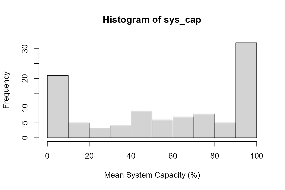
Distribution of system capacity values for temperature at the example location. The spread reflects uncertainty in both the temperature measurement and the dose-response relationship.
At a mean temperature of 14°C, the system capacity is relatively high (around 80%), which matches our dose-response curve where 14°C corresponds to good habitat conditions.
Running the Full Joe Model
Now let’s run the complete Joe Model, which:
- Calculates system capacity for every stressor at every location
- Combines individual stressor effects into a cumulative system capacity score
- Repeats this process across multiple Monte Carlo simulations to quantify uncertainty
Loading the Data
# Load both workbooks
filename_rm <- system.file("extdata", "stressor_magnitude_unc_ARTR.xlsx", package = "CEMPRA")
filename_sr <- system.file("extdata", "stressor_response_fixed_ARTR.xlsx", package = "CEMPRA")

dose <- StressorMagnitudeWorkbook(filename = filename_rm, scenario_worksheet = "natural_unc")
sr_wb_dat <- StressorResponseWorkbook(filename = filename_sr)

# Check how many locations and stressors we have
cat("Number of locations:", length(unique(dose$HUC_ID)), "\n")
#> Number of locations: 103
cat("Number of stressors:", nrow(sr_wb_dat$main_sheet), "\n")
#> Number of stressors: 18
Running the Model
The JoeModel_Run() function handles all the
calculations:
# Run the Joe Model
jmr <- JoeModel_Run(
  dose = dose,           # Stressor magnitude data
  sr_wb_dat = sr_wb_dat, # Stressor-response relationships
  MC_sims = 10           # Number of Monte Carlo simulations (use more for final analysis)
)

# Examine the output structure
names(jmr)
#> [1] "ce.df"      "sc.dose.df"
Handling Missing Stressor Data: strict_na
In real-world datasets, some locations may be missing data for one or
more stressors. The strict_na parameter controls how these
gaps affect the results:
-
strict_na = FALSE(the default): Missing stressor values are treated as having no effect (system capacity = 1 for that stressor). This is a permissive approach — locations are scored based on whatever data is available. -
strict_na = TRUE: Any missing stressor data causes the cumulative score for that location to becomeNA. This is a conservative approach — it flags locations with incomplete data rather than assuming they are unimpacted.
For exploratory analyses the default is usually fine. For formal
assessments where data completeness matters, consider using
strict_na = TRUE so that gaps are visible in the
output:
# Conservative: flag locations with missing stressor data
jmr <- JoeModel_Run(dose = dose, sr_wb_dat = sr_wb_dat, MC_sims = 100, strict_na = TRUE)
Understanding the Output
The Joe Model returns a list with two key components:
| Component | Description |
|---|---|
ce.df |
Cumulative Effects - Overall system capacity for each location and simulation |
sc.dose.df |
Stressor-specific Capacity - System capacity broken down by individual stressor |
Let’s start by visualizing the raw distribution of cumulative system capacity across all locations and simulations:
# Extract cumulative system capacity (as percentage)
msc <- jmr$ce.df$CE * 100

hist(msc,
     xlab = "Cumulative System Capacity (%)",
     main = "Joe Model Results - All Locations",
     col = "steelblue",
     border = "white",
     breaks = 20)
abline(v = mean(msc), col = "red", lwd = 2, lty = 2)
legend("topleft",
       legend = c(paste("Mean =", round(mean(msc), 1), "%"),
                  paste("Min =", round(min(msc), 1), "%"),
                  paste("Max =", round(max(msc), 1), "%")),
       bty = "n")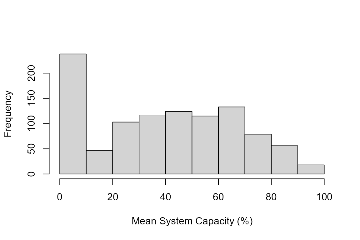
Distribution of cumulative system capacity across all locations and Monte Carlo simulations. Lower values indicate locations where multiple stressors are limiting habitat quality.
Note that this histogram mixes two sources of variation together: spatial differences between locations and Monte Carlo uncertainty within each location. To separate these, we can summarize the results at the location level.
Location-Level Summary
By averaging across Monte Carlo simulations for each location, we can see the spatial pattern — which locations are most impacted by cumulative stressors:
# Calculate mean system capacity per location across MC simulations
loc_means <- tapply(jmr$ce.df$CE, jmr$ce.df$HUC, mean) * 100

# Sort from lowest to highest capacity
loc_means <- sort(loc_means)

# Barplot of location-level means
par(mar = c(5, 4, 3, 1))
bp <- barplot(loc_means,
              xlab = "Location (HUC_ID)",
              ylab = "Mean System Capacity (%)",
              main = "System Capacity by Location",
              col = ifelse(loc_means < 40, "#E8726A",
                    ifelse(loc_means < 70, "#F5C242", "#6AB187")),
              border = NA,
              las = 2,
              cex.names = 0.6,
              ylim = c(0, 100))
abline(h = c(40, 70), col = "grey50", lty = 3)
legend("topleft",
       legend = c("< 40% (heavily impacted)",
                  "40-70% (moderately impacted)",
                  "> 70% (good condition)"),
       fill = c("#E8726A", "#F5C242", "#6AB187"),
       border = NA, bty = "n", cex = 0.85)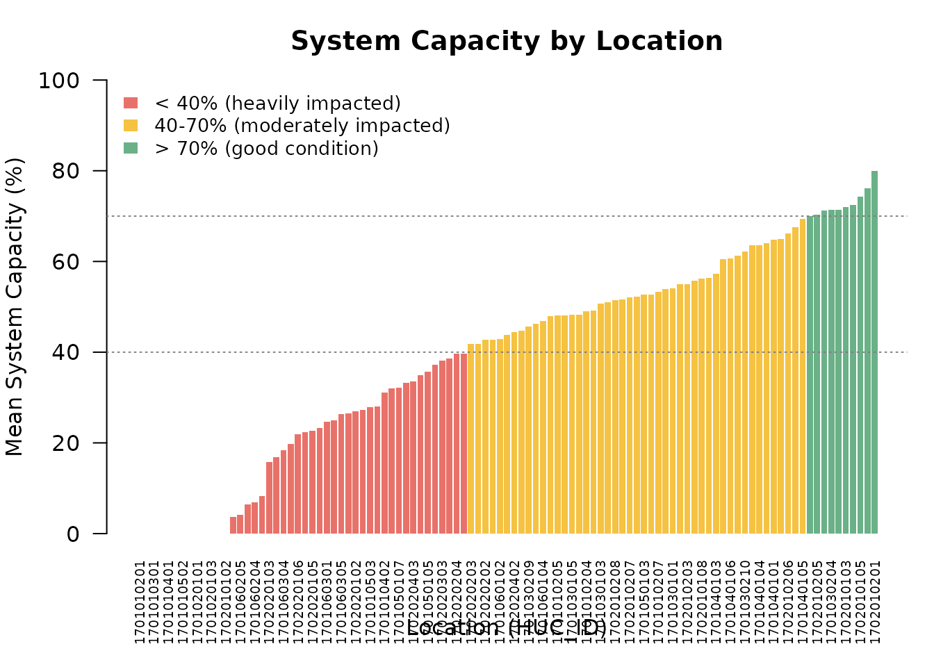
Mean cumulative system capacity for each location, averaged across Monte Carlo simulations. Locations are sorted from most impacted (left) to least impacted (right).
This view makes it easy to identify the most impacted locations that may benefit from targeted recovery actions.
Uncertainty at a Single Location
Next, let’s look at the Monte Carlo uncertainty for one specific location. This shows how confident we are in the system capacity estimate, given uncertainty in both the stressor measurements and the dose-response relationships:
# Pick the location with the lowest mean capacity to examine
target_huc <- names(loc_means)[1]

# Extract MC results for this location
huc_ce <- jmr$ce.df$CE[as.character(jmr$ce.df$HUC) == target_huc] * 100

hist(huc_ce,
     xlab = "Cumulative System Capacity (%)",
     main = paste("MC Uncertainty - Location", target_huc),
     col = "coral",
     border = "white",
     breaks = 15,
     xlim = c(0, 100))
abline(v = mean(huc_ce), col = "darkred", lwd = 2, lty = 2)
abline(v = quantile(huc_ce, c(0.05, 0.95)), col = "grey40", lwd = 1, lty = 3)
legend("topright",
       legend = c(paste("Mean =", round(mean(huc_ce), 1), "%"),
                  paste("90% CI:", round(quantile(huc_ce, 0.05), 1), "-",
                        round(quantile(huc_ce, 0.95), 1), "%")),
       col = c("darkred", "grey40"),
       lty = c(2, 3), lwd = c(2, 1), bty = "n", cex = 0.9)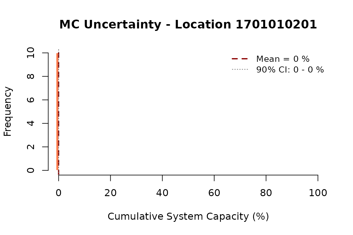
Distribution of cumulative system capacity across Monte Carlo simulations for a single location. The spread reflects combined uncertainty from stressor measurements and dose-response relationships.
Interpreting the Results
These three views give complementary insights:
- Overall histogram: A quick snapshot of the full range of outcomes across all locations and simulations
- Location barplot: The spatial pattern — which locations are most/least impacted, after averaging out MC uncertainty
- Single-location histogram: The uncertainty envelope — how confident we are in the estimate for a given location
As a general guide for the system capacity values:
- High values (>70%): Locations with good habitat conditions where few stressors are limiting
- Medium values (40-70%): Locations where some stressors are degrading habitat quality
- Low values (<40%): Heavily impacted locations where multiple stressors are limiting capacity
Next Steps
This tutorial covered the basics of running the Joe Model for a single scenario. To learn more about:
- Running multiple scenarios: See Tutorial 2: Joe Model Batch Run
- Linking to population dynamics: See Tutorial 3: Population Model Overview
- Sensitivity analysis: See Tutorial 5: Population Model Evaluation
For detailed guidance on preparing your own data, see the CEMPRA Documentation.