3. Population Model Overview

Overview

This tutorial covers the Population Model component of the CEMPRA framework. Building on the Joe Model’s system capacity scores, the population model translates cumulative effects into demographic impacts on a target species. By the end of this tutorial, you will understand how to: - Configure life cycle parameters for a target species - Run stage-structured matrix population projections - Incorporate density-dependent constraints on population growth - Link environmental stressors to vital rates (survival, fecundity, capacity) - Compare population trajectories under baseline vs. cumulative effect scenarios

What is the Population Model?

The population model is a stage-structured matrix model that projects a hypothetical population forward through time. Unlike the Joe Model, which produces a single system capacity score, the population model:

Tracks simulated individuals through multiple life stages (e.g., egg, fry, juvenile, adult)
Applies density-dependent constraints using Beverton-Holt or Hockey-Stick functions based on habitat availability.
Links stressors to vital rates (survival, fecundity, or carrying capacity at specific life stages)
Produces time series projections showing how population abundance changes over years

This allows you to understand which life stages are most limiting and how stressors affect population dynamics.

When to Use the Population Model

Use Case	Benefit
Identify demographic bottlenecks	Understand which life stages limit population growth
Compare recovery scenarios	Evaluate which stressor reductions have the largest population benefit
Assess cumulative effects	See how multiple stressors combine to affect population trajectories
Spatial prioritization	Compare population dynamics across locations

Prerequisites

Before starting this tutorial, you should:

Complete Tutorial 1: Joe Model Overview to understand stressor-response relationships
Have basic familiarity with population ecology concepts (carrying capacity, density dependence)
Review the CEMPRA Guidance Document Section on the Life Cycle Model for detailed background

Installation

# Install CEMPRA from GitHub (if not already installed)
# library(devtools)
# install_github("essatech/CEMPRA")

# Load required packages
library(CEMPRA)
library(ggplot2)

Understanding the Input Data

The population model requires several input files:

Input File	Purpose
Life Cycle Profile (CSV)	Species-specific vital rates: survival, fecundity, maturity schedules
Stressor-Response Workbook (Excel)	Dose-response curves linking stressors to system capacity
Stressor-Magnitude Workbook (Excel)	Location-specific stressor values
Habitat Capacities File (Excel or CSV, optional)	Location and stage-specific carrying capacities

The stressor-response and stressor-magnitude workbooks are the same files used in the Joe Model. The life cycle profile and habitat capacity files are new and specific to population modeling.

Linking Stressors to Vital Rates

A key feature of the population model is the ability to link environmental stressors directly to life-stage-specific vital rates. This is configured in the Stressor-Response Excel Workbook through the Life_stages and Parameters columns on the Main worksheet.

Stressor-Response Workbook Structure

Recall from Tutorial 1 that the stressor-response workbook contains a Main worksheet that indexes all stressors. For the population model, two additional columns are critical (the Life_stages and the Parameters columns):

Example Main worksheet showing Life_stages and Parameters columns
Stressors	Life_stages	Parameters
Fines	egg	survival
Spawn_Gravel	spawners	capacity
Spawn_Quality	spawners	capacity
Wood_Abund_Fry	stage_0	survival
Wood_Abund_Spawn	spawners	capacity
Fry_Capacity	stage_0	capacity

By carefully defining these columns we can effecively link stressor-response relationships to specific vital rates. Each stressor-response relationship can be linked to only one vital rate. If multiple linkages are desired then duplicate the stressor & stressor-response relationship accordingly in the Stressor Magnitude and Stressor-Response workbook (e.g., SummerStreamTemp_Parr, SummerStreamTemp_Prespawn).

The Parameters Column

The in the Stressor-Response workbook Parameters column specifies how the stressor-response relationship affects the vital rate of interest. There are three possible values:

Value	Effect	Description
`capacity`	Reduces carrying capacity	The stressor reduces the maximum number of individuals that habitat can support at the target life stage (K). This affects density-dependent regulation.
`survival`	Reduces survival probability	The stressor directly reduces the survival rate (S) for the target life stage. This is a density-independent effect.
`fecundity`	Reduces reproductive output	The stressor reduces eggs per spawner (eps). Less commonly used.
blank or `NA`	Joe Model only	The stressor contributes to system capacity but is not linked to the population model.

Example interpretation:

A stressor with Parameters = "capacity" and Life_stages = "stage_0" reduces the fry carrying capacity. If the system capacity score is 0.70, the fry capacity (K0) is reduced to 70% of baseline.
A stressor with Parameters = "survival" and Life_stages = "stage_1" reduces stage-1 survival. If the system capacity score is 0.85, the stage-1 survival rate is multiplied by 0.85.

The Life_stages Column

The Life_stages column specifies which life stage(s) (or specific vital rate) the stressor affects. The population model recognizes stage-specific tags and several convenient aliases.

Stage-Specific Tags (Recommended)

For clarity and precision, we recommend using explicit stage numbers:

Survival Tags for Non-Anadromous Populations:

Life_stages Column	Target Vital Rate
`stage_E`, `SE`	Egg survival
`stage_0`, `S0`	Age-0 fry/sub-yearling survival
`stage_1`, `S1`, `surv_1`	Stage 1 survival
`stage_2`, `S2`, `surv_2`	Stage 2 survival
… up to `stage_12`	Higher stages as needed

Capacity Tags:

Tag(s)	Target
`SE`, `stage_E`, `KE`	Egg capacity (Ke)
`stage_0`, `S0`, `K0`	Fry capacity (K0)
`stage_1`, `S1`, `K1`	Stage 1 capacity
`stage_2`, `S2`, `K2`	Stage 2 capacity
… up to `stage_12`	Higher stages as needed

Anadromous-Specific Tags

For anadromous species, additional tags target pre-breeder (Pb) and spawner (Breeder - B) classes:

Pre-breeder Survival (Pb):

Tag(s)	Target
`stage_E`, `SE`	Egg survival
`stage_0`, `S0`	Age-0 fry/sub-yearling survival
`stage_Pb_1`	Pre-breeder stage 1 survival
`stage_Pb_2`	Pre-breeder stage 2 survival
… up to `stage_Pb_12`	Higher stages as needed

Pre-breeder Capacity (Pb):

Tag(s)	Target
`stage_Pb_1`	Pre-breeder stage 1 capacity
`stage_Pb_2`	Pre-breeder stage 2 capacity
… up to `stage_Pb_12`	Higher stages as needed

Spawner Capacity (B):

Tag(s)	Target
`spawners`	All spawner capacity (pooled across ages)
`spawn_1`, `spawners_1`, `B1`, `stage_B_1`	Age-specific spawner capacity
… up to `spawn_12`	Higher ages as needed

Pre-spawn and Migration Survival (Anadromous only):

Tag(s)	Target
`spawners`	All pre-spawn survival (u)
`prespawn_1`, `u1` … `u12`	Age-specific pre-spawn survival
`smig`, `spawn_mig`	All spawner migration survival
`smig_1`, `spawn_mig_1` … `smig_12`	Age-specific migration survival

Fecundity Tags

Tag	Target
`eps`	Eggs per spawner (all ages)
`eps_3`, `eps_4`, …	Age-specific fecundity (anadromous)

Notes on Life Stage Tags

Tags are case-insensitive (converted to lowercase internally)
Underscores and spaces are removed during processing (e.g., stage_1 and stage1 are equivalent)
You can specify multiple life stages separated by commas (e.g., stage_1, stage_2)
We recommend using explicit stage numbers (stage_1, stage_2) rather than legacy nicknames for clarity

Part 1: Non-Anadromous Populations

We’ll start with a non-anadromous (resident) species because the life cycle structure is simpler. The example uses parameters representative of Westslope Cutthroat Trout or similar resident trout species. Use the non-anadromous mode for all resident trout or iteroparous species.

1.1 Loading Example Data

Let’s load the example life cycle profile included with CEMPRA:

# Load the life cycle parameters file
filename_lc <- system.file("extdata", "life_cycles.csv", package = "CEMPRA")
life_cycles <- read.csv(filename_lc)

# View the parameters
print(life_cycles)
#>                                              Parameters    Name  Value
#> 1                                 Number of life stages  Nstage    4.0
#> 2                                        Adult capacity       k  100.0
#> 3                               Spawn events per female  events    1.0
#> 4                                 Eggs per female spawn     eps 3000.0
#> 5                                     spawning interval     int    1.0
#> 6                                          egg survival      SE    0.1
#> 7                                          yoy survival      S0    0.3
#> 8                                             sex ratio      SR    0.5
#> 9                                    Hatchling Survival  surv_1    0.3
#> 10                                    Juvenile Survival  surv_2    0.3
#> 11                                   Sub-adult Survival  surv_3    0.9
#> 12                                       Adult Survival  surv_4    0.9
#> 13                                   Years as hatchling  year_1    1.0
#> 14                                    years as juvenile  year_2    2.0
#> 15                                    years as subadult  year_3    2.0
#> 16                                       years as adult  year_4    5.0
#> 17                      egg survival compensation ratio    cr_E    1.0
#> 18                      yoy survival compensation ratio    cr_0    3.0
#> 19                hatchling survival compensation ratio    cr_1    2.5
#> 20                 juvenile survival compensation ratio    cr_2    2.0
#> 21                 subadult survival compensation ratio    cr_3    1.1
#> 22                    adult survival compensation ratio    cr_4    1.0
#> 23                                maturity as hatchling   mat_1    0.0
#> 24                                 maturity as juvenile   mat_2    0.0
#> 25                                 maturity as subadult   mat_3    0.0
#> 26                                    maturity as adult   mat_4    1.0
#> 27                          variance in eggs per female  eps_sd 1000.0
#> 28            correlation in egg fecundity through time egg_rho    0.1
#> 29 coefficient of variation in stage-specific mortality    M.cv    0.1
#> 30                correlation in mortality through time   M.rho    0.1

1.2 Understanding the Life Cycle Profile

The life cycle profile is a CSV file with three columns:

Column	Description
Parameters	Human-readable description (can be customized nickname)
Name	Parameter code used by the model (do not modify)
Value	Numeric value for the parameter

Key Parameter Groups

Population Structure:

Parameters	Name	Value
Number of life stages	Nstage	4
Adult capacity	k	100

Nstage: Number of life stages (excluding egg/fry stage 0)
k: (OPTIONAL) Adult carrying capacity (used with compensation ratios)

Survival Rates:

Parameters	Name	Value
egg survival	SE	0.1
yoy survival	S0	0.3
sex ratio	SR	0.5
Hatchling Survival	surv_1	0.3
Juvenile Survival	surv_2	0.3
Sub-adult Survival	surv_3	0.9
Adult Survival	surv_4	0.9

SE: Egg survival (density-independent)
S0: Age-0 fry/sub-yearling survival (density-independent)
surv_1 to surv_N: Stage-specific annual survival rates

Important: These survival values should represent density-independent survival (i.e., maximum survival in the absence of crowding). Density-dependent effects are applied separately.

Years in Each Stage:

Parameters	Name	Value
Years as hatchling	year_1	1
years as juvenile	year_2	2
years as subadult	year_3	2
years as adult	year_4	5

year_1 to year_N: Number of years individuals spend in each stage
If all values are 1, this is an age-based (Leslie) matrix model
Values > 1 allow individuals to remain in a stage for multiple years (stage-based model)

Fecundity:

Parameters	Name	Value
Spawn events per female	events	1e+00
Eggs per female spawn	eps	3e+03
spawning interval	int	1e+00
sex ratio	SR	5e-01

events: Spawning events per female per year (typically 1)
eps: Eggs per female spawner
int: Spawning interval in years (typically 1)
SR: Sex ratio (proportion female, typically 0.5)

Maturity Schedule:

Parameters	Name	Value
maturity as hatchling	mat_1	0
maturity as juvenile	mat_2	0
maturity as subadult	mat_3	0
maturity as adult	mat_4	1

mat_1 to mat_N: Proportion of each stage that is sexually mature (0-1)
In this example, only stage 4 adults are mature (mat_4 = 1)

Stochasticity Parameters:

Parameters	Name	Value
variance in eggs per female	eps_sd	1e+03
correlation in egg fecundity through time	egg_rho	1e-01
coefficient of variation in stage-specific mortality	M.cv	1e-01
correlation in mortality through time	M.rho	1e-01

eps_sd: Standard deviation in eggs per female
egg_rho: Correlation in fecundity between years (0-1)
M.cv: Coefficient of variation in stage-specific mortality
M.rho: Correlation in mortality between years (0-1)

Higher correlation values mean good/bad years affect all cohorts simultaneously.

1.3 Setting Up the Matrix Model

The population model uses two setup functions to build the mathematical framework:

# Step 1: Initialize population model parameters
pop_mod_setup <- pop_model_setup(life_cycles = life_cycles)

# Step 2: Build matrix elements
pop_mod_mat <- pop_model_matrix_elements(pop_mod_setup = pop_mod_setup)
#> Running with S0 adjusted to s0.1.det...

# View the components created
names(pop_mod_mat)
#> [1] "projection_matrix"      "life_histories"         "life_stages_symbolic"  
#> [4] "density_stage_symbolic" "anadrmous"

The pop_model_matrix_elements() function returns:

projection_matrix: The numerical transition matrix (A)
life_stages_symbolic: Symbolic (equation) form of the matrix
density_stage_symbolic: Density-dependence modifier matrix
life_histories: Derived life history parameters

The Transition Matrix

The transition matrix governs how individuals move between life stages:

# View the transition matrix
A <- pop_mod_mat$projection_matrix
print(round(A, 3))
#>      [,1]  [,2]  [,3]   [,4]
#> [1,]  0.0 0.000 0.000 45.000
#> [2,]  0.3 0.231 0.000  0.000
#> [3,]  0.0 0.069 0.474  0.000
#> [4,]  0.0 0.000 0.426  0.756

Reading the matrix:

Rows represent the “to” stage; columns represent the “from” stage
The top row contains fecundity elements (new recruits from mature stages)
The diagonal elements represent probability of staying in the same stage
Sub-diagonal elements represent probability of advancing to the next stage

1.4 Eigenanalysis (Density-Independent Growth)

Before running full projections, we can use eigenanalysis to understand basic population dynamics under density-independent conditions:

# Calculate lambda (intrinsic growth rate)
lambda_val <- popbio::lambda(A)
cat("Lambda (intrinsic growth rate):", round(lambda_val, 3), "\n")
#> Lambda (intrinsic growth rate): 1.211

# Lambda > 1 means population grows exponentially
# Lambda < 1 means population declines
# Lambda = 1 means stable population

# Calculate elasticities (proportional sensitivity)
eigen_results <- popbio::eigen.analysis(A)
print("Elasticities:")
#> [1] "Elasticities:"
print(round(eigen_results$elasticities, 3))
#>       [,1]  [,2]  [,3]  [,4]
#> [1,] 0.000 0.000 0.000 0.153
#> [2,] 0.153 0.036 0.000 0.000
#> [3,] 0.000 0.153 0.098 0.000
#> [4,] 0.000 0.000 0.153 0.254

Interpreting elasticities: Elasticities show which matrix elements have the greatest proportional influence on lambda. Higher values indicate life stages where changes have the largest impact on population growth.

1.5 Running Density-Dependent Projections

Real populations don’t grow exponentially forever - they experience density-dependent constraints. The Projection_DD() function projects the population forward while applying these constraints.

Basic Projection (No Stressors)

# Extract the components needed for projection
life_histories <- pop_mod_mat$life_histories
life_stages_symbolic <- pop_mod_mat$life_stages_symbolic
density_stage_symbolic <- pop_mod_mat$density_stage_symbolic

# Run population projection for 100 years
baseline <- Projection_DD(
  M.mx = life_stages_symbolic,       # Transition matrix (symbolic)
  D.mx = density_stage_symbolic,     # Density-dependence matrix
  H.mx = NULL,                       # Harvest matrix (not used)
  dat = life_histories,              # Life history parameters
  K = life_histories$Ka,             # Adult carrying capacity
  Nyears = 100,                      # Years to simulate
  p.cat = 0,                         # Probability of catastrophe
  CE_df = NULL                       # No cumulative effect stressors
)

# View the output components
names(baseline)
#> [1] "pop"     "N"       "lambdas" "vars"    "Cat."

# Plot population trajectory
plot(baseline$pop$year, baseline$pop$N,
     type = 'l', lwd = 2, col = "darkblue",
     xlab = "Year", ylab = "Total Population (N)",
     main = "Baseline Population Projection (No Stressors)")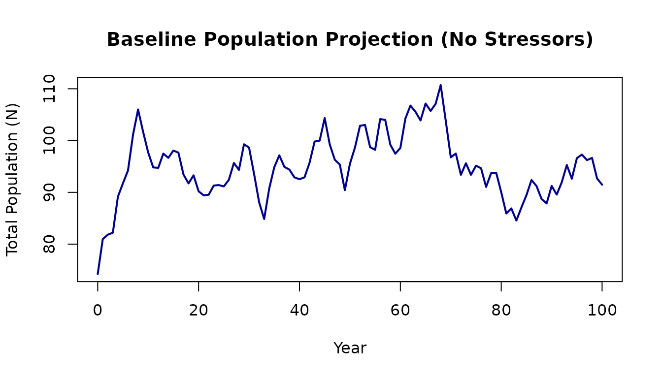

The population fluctuates around the carrying capacity due to stochastic variation in survival and fecundity.

Understanding Density Dependence

The model uses Beverton-Holt density dependence by default. This creates a compensatory relationship where survival decreases as population density approaches carrying capacity:

$N_{t+1} = \frac{S \cdot N_t}{1 + \frac{(S-1) \cdot N_t}{K}}$

Where: - $S$ = density-independent survival rate - $N_t$ = current population size - $K$ = carrying capacity

The model also supports Hockey-Stick density dependence, which imposes a hard cap at carrying capacity.

1.6 Adding Cumulative Effect Stressors

Now let’s add environmental stressors that affect population vital rates. Stressors can target:

survival: Reduces survival probability for specific life stages
capacity: Reduces carrying capacity for specific life stages

Creating a Simple Stressor Dataset

# Create stressor data for a hypothetical location
# Stressor 1: Reduces fry carrying capacity by 58%
CE_df1 <- data.frame(
  HUC = 123,
  Stressor = "Temperature",
  dose = 20,              # Stressor magnitude (e.g., 20 deg C)
  sys.cap = 0.42,         # 42% of baseline capacity remains
  life_stage = "stage_0",
  parameter = "capacity",
  Stressor_cat = "Temperature"
)

# Stressor 2: Reduces stage-1 survival by 20%
CE_df2 <- data.frame(
  HUC = 123,
  Stressor = "Sediment",
  dose = 30,              # Stressor magnitude (e.g., 30% fines)
  sys.cap = 0.80,         # 80% of baseline survival remains
  life_stage = "stage_1",
  parameter = "survival",
  Stressor_cat = "Sediment"
)

# Combine stressors
CE_df <- rbind(CE_df1, CE_df2)
print(CE_df)
#>   HUC    Stressor dose sys.cap life_stage parameter Stressor_cat
#> 1 123 Temperature   20    0.42    stage_0  capacity  Temperature
#> 2 123    Sediment   30    0.80    stage_1  survival     Sediment

1.7 Comparing Baseline vs. CE Scenarios

Now let’s run the projection with stressors and compare to baseline:

# Run projection WITH cumulative effect stressors
ce_projection <- Projection_DD(
  M.mx = life_stages_symbolic,
  D.mx = density_stage_symbolic,
  H.mx = NULL,
  dat = life_histories,
  K = life_histories$Ka,
  Nyears = 100,
  p.cat = 0,
  CE_df = CE_df
)

# Plot comparison
plot(baseline$pop$year, baseline$pop$N,
     type = 'l', lwd = 2, col = "black",
     xlab = "Year", ylab = "Total Population (N)",
     main = "Population Projection: Baseline vs. Cumulative Effects",
     ylim = c(0, max(baseline$pop$N) * 1.1))
lines(ce_projection$pop$year, ce_projection$pop$N,
      lwd = 2, col = "red")
legend("topright",
       legend = c("Baseline", "With Stressors"),
       col = c("black", "red"), lwd = 2, bty = "n")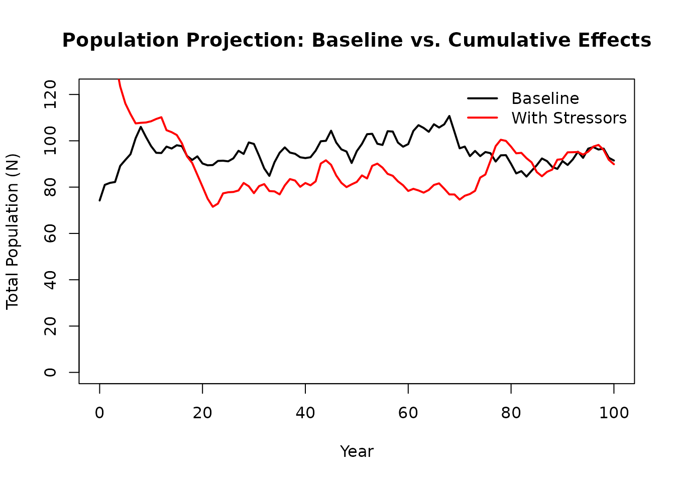


# Calculate relative impact
baseline_median <- median(baseline$pop$N[50:100])
ce_median <- median(ce_projection$pop$N[50:100])
relative_capacity <- ce_median / baseline_median

cat("\nBaseline median abundance:", round(baseline_median, 0))
#> 
#> Baseline median abundance: 96
cat("\nWith stressors median abundance:", round(ce_median, 0))
#> 
#> With stressors median abundance: 87
cat("\nRelative system capacity:", round(relative_capacity * 100, 1), "%\n")
#> 
#> Relative system capacity: 90.5 %

The red line shows population suppression when environmental stressors are applied.

1.8 Using Location-Specific Habitat Capacities

For more realistic modeling, you can specify location and stage-specific carrying capacities instead of (or in addition to) using compensation ratios.

Habitat Capacity File Format

# View the example habitat capacity file structure
filename_dd <- system.file("extdata", "habitat_dd_k.xlsx", package = "CEMPRA")
habitat_dd_k <- readxl::read_excel(filename_dd)
print(as.data.frame(habitat_dd_k[1:3, ]))
#>   HUC_ID NAME k_stage_0_mean k_stage_1_mean k_stage_2_mean k_stage_3_mean
#> 1      1   NA          10000          1e+07          1e+07          1e+05
#> 2      2   NA             NA             NA             NA             NA
#> 3      3   NA             NA             NA             NA             NA
#>   k_stage_4_mean k_stage_0_cv k_stage_1_cv k_stage_2_cv k_stage_3_cv
#> 1           1000          0.1          0.1          0.1          0.1
#> 2             NA           NA           NA           NA           NA
#> 3             NA           NA           NA           NA           NA
#>   k_stage_4_cv notes
#> 1          0.1    NA
#> 2           NA    NA
#> 3           NA    NA

The habitat capacity file has columns:

Column	Description
`HUC_ID`	Location identifier (must match stressor data)
`NAME`	Location name
`k_stage_0_mean`	Carrying capacity for fry (stage 0)
`k_stage_1_mean`	Carrying capacity for stage 1
`k_stage_2_mean`, etc.	Carrying capacity for subsequent stages
`k_stage_X_cv`	(Optional) Coefficient of variation for interannual variability

Important: Only include columns for stages with density-dependent bottlenecks. Leave cells blank or omit columns for stages without capacity constraints.

Enabling Stage-Specific Density Dependence

To use stage-specific capacities, you must add density-dependence flags to your life cycle profile:

# Add these rows to your life_cycles.csv to enable density dependence:
# Name         Value
# bh_stage_0   TRUE    # Beverton-Holt for egg-to-fry transition
# bh_stage_1   TRUE    # Beverton-Holt for fry-to-parr transition
# hs_stage_2   TRUE    # Hockey-Stick for stage 2 (hard cap)

Flag	Function	Description
`bh_stage_0`	Beverton-Holt	Egg-to-fry transition
`hs_stage_0`	Hockey-Stick	Egg-to-fry (hard cap)
`bh_stage_1`, `bh_stage_2`, …	Beverton-Holt	Stage transitions
`hs_stage_1`, `hs_stage_2`, …	Hockey-Stick	Stage transitions (hard cap)

Part 2: Anadromous Populations

Anadromous species (salmon) require a different model structure because:

Individuals spawn only once and then die (semelparity)
Fish may return to spawn at different ages (age-3, age-4, age-5)
The model must track pre-breeders (fish still at sea) separately from breeders (returning spawners)

2.1 Key Differences from Non-Anadromous Models

Feature	Non-Anadromous	Anadromous
Spawning	Multiple times (iteroparous)	Once then die (semelparous)
Maturity	Single stage matures	Multiple age classes can mature
Structure	Stages can span multiple years	Each year is typically one stage
Parameters	Single `eps`	Age-specific `eps_3`, `eps_4`, `eps_5`
Additional rates	None	Migration survival (`smig_X`), pre-spawn survival (`u_X`)

2.2 Loading Anadromous Example Data (Nanaimo Chinook)

For this example, we’ll use a complete dataset for Chinook Salmon from the Nanaimo River system. This includes the life cycle profile, stressor data, and habitat capacities:

# Load anadromous life cycle profile
filename_lc_anad <- system.file("extdata", "nanaimo/species_profiles/nanaimo_comp_ocean_summer.csv", package = "CEMPRA")
life_cycles_anad <- read.csv(filename_lc_anad)

# Load stressor-response workbook
filename_sr_anad <- system.file("extdata", "nanaimo/stressor_response_nanaimo.xlsx", package = "CEMPRA")
sr_wb_anad <- StressorResponseWorkbook(filename = filename_sr_anad)

# Load stressor-magnitude workbook
filename_sm_anad <- system.file("extdata", "nanaimo/stressor_magnitude_nanaimo.xlsx", package = "CEMPRA")
dose_anad <- StressorMagnitudeWorkbook(filename = filename_sm_anad)

# Load habitat capacities file
filename_hab_anad <- system.file("extdata", "nanaimo/habitat_capacities_nanaimo.csv", package = "CEMPRA")
habitat_dd_k_anad <- read.csv(filename_hab_anad)

# View available locations
print(unique(dose_anad$HUC_ID))
#> [1] 1 2 3

2.3 Understanding the Anadromous Life Cycle Profile

# View key parameters
print(life_cycles_anad)
#>                                              Parameters          Name  Value
#> 1                                 Number of life stages        Nstage      5
#> 2                                            Anadromous    anadromous   TRUE
#> 3                                        Adult capacity             k   5000
#> 4                               Spawn events per female        events      1
#> 5                         Eggs per age-3 female spawner         eps_3   1953
#> 6                         Eggs per age-4 female spawner         eps_4   4000
#> 7                         Eggs per age-5 female spawner         eps_5   5200
#> 8                                     Spawning interval           int      1
#> 9                                          Egg survival            SE    0.4
#> 10                                         Fry survival            S0    0.4
#> 11                             Sex ratio male to female            SR    0.5
#> 12                                   Stage 1 to Stage 2        surv_1 0.0498
#> 13                                   Stage 2 to Stage 3        surv_2    0.7
#> 14                                   Stage 3 to Stage 4        surv_3    0.8
#> 15                                   Stage 4 to Stage 5        surv_4    0.9
#> 16                                   Stage 5 to Stage 6        surv_5      0
#> 17                Pre-spawn mortality of Age-3 spawners           u_3      1
#> 18                Pre-spawn mortality of Age-4 spawners           u_4      1
#> 19                Pre-spawn mortality of Age-5 spawners           u_5      1
#> 20                Pre-spawn mortality of Age-6 spawners           u_6      1
#> 21                 Migration survival of Age-3 spawners        smig_3    0.9
#> 22                 Migration survival of Age-4 spawners        smig_4    0.9
#> 23                 Migration survival of Age-5 spawners        smig_5    0.9
#> 24                       compensation ratios - not used          cr_E      1
#> 25                       compensation ratios - not used          cr_0      1
#> 26                       compensation ratios - not used          cr_1      1
#> 27                       compensation ratios - not used          cr_2      1
#> 28                       compensation ratios - not used          cr_3      1
#> 29                       compensation ratios - not used          cr_4      1
#> 30                       compensation ratios - not used          cr_5      1
#> 31                     probability of maturity at age-3         mat_3    0.2
#> 32                     probability of maturity at age-4         mat_4    0.6
#> 33                     probability of maturity at age-5         mat_5      1
#> 34                          variance in eggs per female        eps_sd    500
#> 35            correlation in egg fecundity through time       egg_rho    0.1
#> 36 coefficient of variation in stage-specific mortality          M.cv    0.2
#> 37                correlation in mortality through time         M.rho    0.1
#> 38           DD constraint on fry colonization in river    bh_stage_0   TRUE
#> 39              DD constraint on fry rearing in estuary bh_stage_pb_1   TRUE
#> 40     Density-dependent constraint on fry colonization   bh_spawners   TRUE
#>                                                                  Notes
#> 1                                        Max possible spawner age is 6
#> 2                                                                     
#> 3                                                             Not used
#> 4                                                                     
#> 5                                    Avg. from Walters and Korman 2024
#> 6                                           Fix at 4000 from RAMS 2021
#> 7                                    Avg. from Walters and Korman 2024
#> 8                                    Spanwing events occur every year.
#> 9                 Avg. upper lim from RAMs & Walters and Korman (2024)
#> 10                Avg. upper lim from RAMs & Walters and Korman (2024)
#> 11                                          Equal portions male/female
#> 12                        from Walters and Korman et al., 2024: Review
#> 13                                From Beechie et al., 2021 & W&K 2024
#> 14                                From Beechie et al., 2021 & W&K 2024
#> 15                                From Beechie et al., 2021 & W&K 2024
#> 16                                                      Terminal stage
#> 17                                                                    
#> 18                                                                    
#> 19                                                                    
#> 20                                                                    
#> 21                                                                    
#> 22                                                                    
#> 23                                                                    
#> 24                                                                    
#> 25                                                                    
#> 26                                                                    
#> 27                                                                    
#> 28                                                                    
#> 29                                                                    
#> 30                                                                    
#> 31 Assume 20% from Walters and Korman avg. of East Coast VI Chin Pops.
#> 32 Assume 20% from Walters and Korman avg. of East Coast VI Chin Pops.
#> 33                                Assume 100% remaining spawn at age-5
#> 34                                                                    
#> 35                                                                    
#> 36                                                    Previouslly 0.02
#> 37                                                                    
#> 38                                                       Beverton-Holt
#> 39                                      Beverton-Holt (but set to inf)
#> 40                                                       Beverton-Holt

The Anadromous Flag

The most important parameter is the anadromous flag:

Parameters	Name	Value
Anadromous	anadromous	TRUE

Setting anadromous = TRUE tells the model to use the anadromous matrix structure.

Age-Specific Fecundity

Unlike non-anadromous models with a single eps value, anadromous models specify fecundity by age:

Parameters	Name	Value
Eggs per age-3 female spawner	eps_3	1953
Eggs per age-4 female spawner	eps_4	4000
Eggs per age-5 female spawner	eps_5	5200

Older fish typically produce more eggs, so age-specific fecundity captures this biological reality.

Age-Specific Maturity Schedule

The maturity schedule determines what proportion of fish return to spawn at each age:

Parameters	Name	Value
probability of maturity at age-3	mat_3	0.2
probability of maturity at age-4	mat_4	0.6
probability of maturity at age-5	mat_5	1

In this example: - 20% of surviving fish spawn at age 3 - 60% of surviving fish spawn at age 4 - 100% of remaining fish spawn at age 5 (maximum age)

Migration and Pre-Spawn Survival

Anadromous models include additional survival parameters:

Parameters	Name	Value
Pre-spawn mortality of Age-3 spawners	u_3	1
Pre-spawn mortality of Age-4 spawners	u_4	1
Pre-spawn mortality of Age-5 spawners	u_5	1
Pre-spawn mortality of Age-6 spawners	u_6	1
Migration survival of Age-3 spawners	smig_3	0.9
Migration survival of Age-4 spawners	smig_4	0.9
Migration survival of Age-5 spawners	smig_5	0.9

smig_X: Migration survival for age-X spawners returning from ocean
u_X: Pre-spawn survival for age-X spawners (survival from arrival to spawning)

Density-Dependence Flags

Note the density-dependence flags at the bottom of the life cycle profile:

Parameters	Name	Value
DD constraint on fry colonization in river	bh_stage_0	TRUE
DD constraint on fry rearing in estuary	bh_stage_pb_1	TRUE
Density-dependent constraint on fry colonization	bh_spawners	TRUE

These flags tell the model which life stages have density-dependent constraints.

2.4 Habitat Capacities for Anadromous Populations

Let’s examine the habitat capacities file:

print(habitat_dd_k_anad)
#>   HUC_ID           NAME k_stage_0_mean k_stage_Pb_1_mean k_stage_B_mean
#> 1      1     Fall Lower         627594                NA          38073
#> 2      2 Summer - Lower        1247555                NA          15384
#> 3      3 Summer - Upper         913589                NA          20943

The habitat capacity file for anadromous species uses column names that distinguish between pre-breeders (Pb) and breeders (B):

Column	Description
`HUC_ID`	Location identifier
`NAME`	Location name
`k_stage_0_mean`	Fry capacity
`k_stage_Pb_1_mean`	Pre-breeder stage 1 capacity (e.g., parr)
`k_stage_B_mean` or `k_spawner_mean`	Total spawner capacity (all ages)

In this example, we have fry capacity (k_stage_0_mean) and spawner capacity (k_stage_B_mean) specified for each location.

2.5 Running the Anadromous Population Model

Now let’s run the full population model for an anadromous species with habitat capacities:

# Select a target location
target_HUC_anad <- 1  # "Fall Lower" population

# Run the population model
results_anad <- PopulationModel_Run(
  dose = dose_anad,
  sr_wb_dat = sr_wb_anad,
  life_cycle_params = life_cycles_anad,
  HUC_ID = target_HUC_anad,
  n_years = 100,
  MC_sims = 5,
  output_type = "adults",
  habitat_dd_k = habitat_dd_k_anad
)

# View output structure
head(results_anad)
#>   year         N MC_sim group
#> 1    0 38073.000      1    ce
#> 2    1  2247.734      1    ce
#> 3    2  6589.878      1    ce
#> 4    3  4434.686      1    ce
#> 5    4  7671.632      1    ce
#> 6    5  1014.496      1    ce

# Calculate summary statistics
baseline_spawners <- median(results_anad$N[results_anad$group == "baseline"], na.rm = TRUE)
ce_spawners <- median(results_anad$N[results_anad$group == "ce"], na.rm = TRUE)

cat("\nBaseline median spawners:", round(baseline_spawners, 0))
#> 
#> Baseline median spawners: 5274
cat("\nWith stressors median spawners:", round(ce_spawners, 0))
#> 
#> With stressors median spawners: 1177
cat("\nRelative capacity:", round(ce_spawners / baseline_spawners * 100, 1), "%\n")
#> 
#> Relative capacity: 22.3 %

Visualizing Anadromous Population Projections

# Plot the results
ggplot(results_anad, aes(x = year, y = N, color = group)) +
  stat_smooth(method = "loess", span = 0.2, se = TRUE,
              aes(fill = group), alpha = 0.3) +
  scale_color_manual(values = c("baseline" = "darkgreen", "ce" = "orange"),
                     labels = c("baseline" = "Baseline", "ce" = "With Stressors")) +
  scale_fill_manual(values = c("baseline" = "darkgreen", "ce" = "orange"),
                    labels = c("baseline" = "Baseline", "ce" = "With Stressors")) +
  labs(x = "Year", y = "Spawner Abundance",
       title = "Anadromous Population Model: Nanaimo Chinook",
       subtitle = paste("Location:", habitat_dd_k_anad$NAME[target_HUC_anad])) +
  theme_bw() +
  theme(legend.position = "bottom",
        legend.title = element_blank())
#> `geom_smooth()` using formula = 'y ~ x'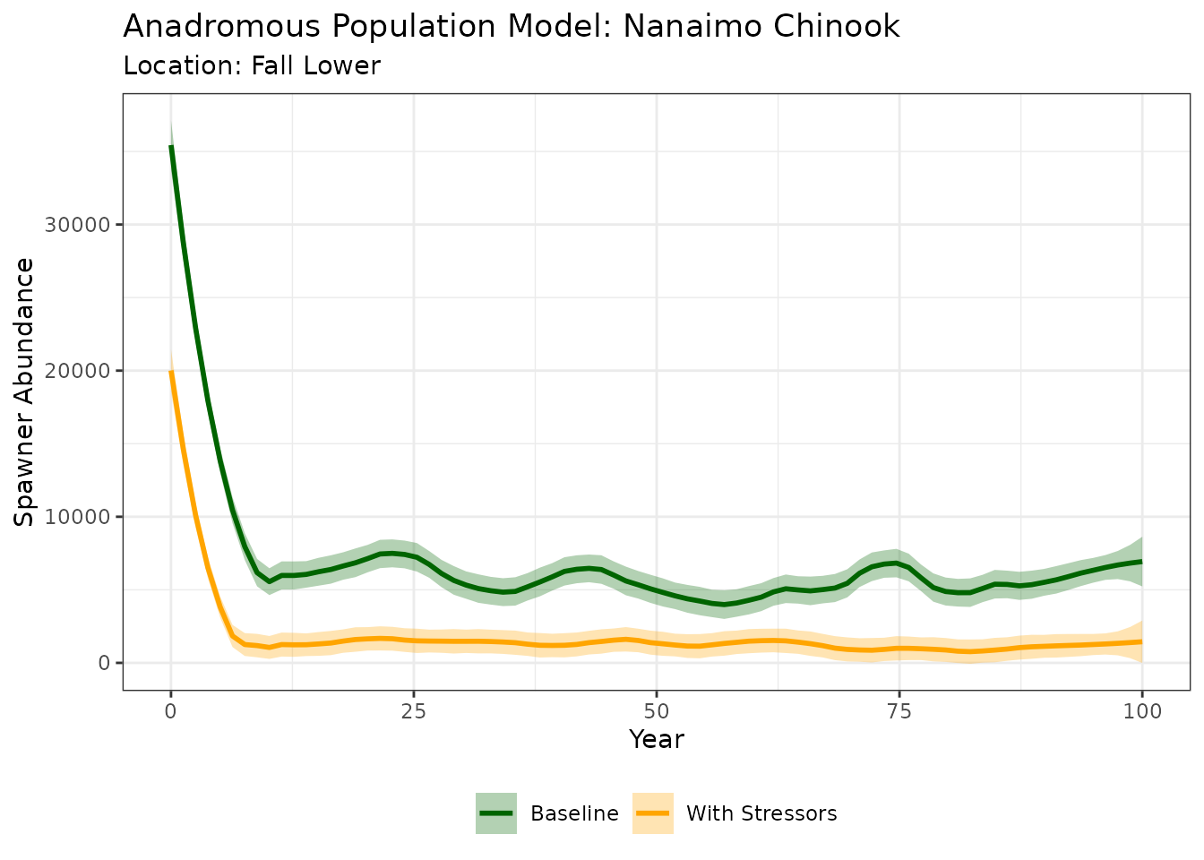

2.6 Comparing Multiple Anadromous Locations

We can run the model for multiple locations and compare outcomes:

# Run for all locations
all_results <- list()

for (huc in unique(dose_anad$HUC_ID)) {
  result <- PopulationModel_Run(
    dose = dose_anad,
    sr_wb_dat = sr_wb_anad,
    life_cycle_params = life_cycles_anad,
    HUC_ID = huc,
    n_years = 100,
    MC_sims = 3,
    output_type = "adults",
    habitat_dd_k = habitat_dd_k_anad
  )
  result$location <- habitat_dd_k_anad$NAME[habitat_dd_k_anad$HUC_ID == huc]
  all_results[[as.character(huc)]] <- result
}

# Combine results
combined_results <- do.call(rbind, all_results)

# Calculate relative capacity by location
location_summary <- aggregate(
  N ~ location + group,
  data = combined_results[combined_results$year > 50, ],
  FUN = median, na.rm = TRUE
)

# Reshape for comparison
library(reshape2)
location_wide <- dcast(location_summary, location ~ group, value.var = "N")
location_wide$relative_capacity <- location_wide$ce / location_wide$baseline * 100

print(location_wide)
#>         location baseline        ce relative_capacity
#> 1     Fall Lower 5119.474 1054.9640         20.606885
#> 2 Summer - Lower 8403.093  833.3773          9.917507
#> 3 Summer - Upper 7746.833  383.4239          4.949428

Running the Full Population Model (Non-Anadromous)

The PopulationModel_Run() function provides a convenient wrapper that:

Runs the Joe Model to calculate stressor effects
Links stressor effects to vital rates by life stage
Runs population projections with and without stressors
Returns comparative results

# Load all required data
filename_sr <- system.file("extdata", "stressor_response_fixed_ARTR.xlsx", package = "CEMPRA")
filename_rm <- system.file("extdata", "stressor_magnitude_unc_ARTR.xlsx", package = "CEMPRA")
filename_lc <- system.file("extdata", "life_cycles.csv", package = "CEMPRA")

sr_wb_dat <- StressorResponseWorkbook(filename = filename_sr)
dose <- StressorMagnitudeWorkbook(filename = filename_rm, scenario_worksheet = "natural_unc")
life_cycle_params <- read.csv(filename_lc)

# Choose a location
target_HUC <- dose$HUC_ID[1]

# Run the population model
results <- PopulationModel_Run(
  dose = dose,
  sr_wb_dat = sr_wb_dat,
  life_cycle_params = life_cycle_params,
  HUC_ID = target_HUC,
  n_years = 100,
  MC_sims = 5,
  output_type = "adults"
)
#> At least one NA in stressor values array
#> Running with S0 adjusted to s0.1.det...

# View output structure
head(results)
#>   year        N MC_sim group
#> 1    0 105.7741      1    ce
#> 2    1 109.4446      1    ce
#> 3    2 107.4242      1    ce
#> 4    3 109.3471      1    ce
#> 5    4 106.8963      1    ce
#> 6    5 104.1837      1    ce

# Plot results
ggplot(results, aes(x = year, y = N, color = group)) +
  stat_smooth(method = "loess", span = 0.2, se = TRUE,
              aes(fill = group), alpha = 0.3) +
  scale_color_manual(values = c("baseline" = "black", "ce" = "red"),
                     labels = c("baseline" = "Baseline", "ce" = "With Stressors")) +
  scale_fill_manual(values = c("baseline" = "black", "ce" = "red"),
                    labels = c("baseline" = "Baseline", "ce" = "With Stressors")) +
  labs(x = "Year", y = "Adult Abundance",
       title = "Population Model: Baseline vs. Cumulative Effects") +
  theme_bw() +
  theme(legend.position = "bottom",
        legend.title = element_blank())
#> `geom_smooth()` using formula = 'y ~ x'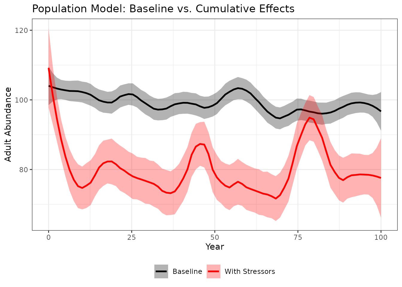

Advanced Topics

Stochasticity Parameters

Control population variability through these parameters:

Parameter	Effect	Typical Values
`eps_sd`	SD in eggs per female	500-1000
`egg_rho`	Correlation in fecundity between years	0.1-0.5
`M.cv`	CV in stage-specific mortality	0.1-0.2
`M.rho`	Correlation in mortality between years	0.1-0.5

Higher correlation values (egg_rho, M.rho) create more synchronized good/bad years across cohorts, increasing population volatility.

Compensation Ratios

Compensation ratios are an alternative way to parameterize density dependence. They modify survival based on how far the population is from carrying capacity:

$S_{adjusted} = \frac{S_{baseline} \cdot K}{K + (CR - 1) \cdot N_t}$

Where CR is the compensation ratio. Higher CR values create stronger density dependence.

Note: We recommend using stage-specific habitat capacities instead of compensation ratios for most applications, as they are more intuitive and directly linked to habitat data.

Probability of Catastrophe

The p.cat parameter models the probability of a catastrophic event (e.g., disease outbreak, extreme flood) that dramatically reduces population:

# Add to life cycle profile:
# p.cat    0.05    # 5% probability of catastrophe per generation

Next Steps

Tutorial	Description
4. Population Model Batch Run	Run population projections across multiple scenarios and locations
5. BC CEF Data Import	Import data from BC Cumulative Effects Framework
6. Population Model Sensitivity	Sensitivity analysis and model evaluation

For additional guidance on building custom species profiles and detailed parameter descriptions, see the CEMPRA Documentation.

References

Caswell, H. (1997). Matrix Methods for Population Analysis. In Structured-Population Models in Marine, Terrestrial, and Freshwater Systems (pp. 19-58).
Van der Lee, A.S. and Koops, M.A. (2020). Recovery Potential Modelling of Westslope Cutthroat Trout. DFO Can. Sci. Advis. Sec. Res. Doc. 2020/046.
Davison, R.J. & Satterthwaite, W.H. (2016). Life cycle models for Pacific salmon. In Pacific Salmon Life Histories (pp. 167-196).
Schaub, M. & Kery, M. (2021). Integrated Population Models: Theory and Ecological Applications with R and JAGS. Academic Press.

2026-01-13